Optimal Transport in Generative Modeling, Part I

I am starting this series for a very practical reason. Recently I’ve been working on flow matching and, in my own reading and experiments, I kept running into papers that said things like “optimal transport (OT) flows straight,” etc. It’s nice to witness the re-revival of OT in deep learning, but many explanations jumped too quickly from buzzwords to conclusions. So that’s why I want to rebuild the story from the ground up, starting from the mathematical object these papers actually use: the coupling.

This first post has only one goal:

explain what a coupling is, what quadratic optimal transport does to couplings, and why that matters later for generative modeling.

I will assume no OT background.

1. The basic generative setup

In generative modeling, we usually start from a simple distribution and want to transform it into a complicated one. Let

$$X_0 \sim q_0, \qquad X_1 \sim q_1.$$

Here:

• $q_0$ is the source distribution, usually something simple like a Gaussian;
• $q_1$ is the target distribution, usually the data distribution.

So the problem is:

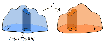
How do we move samples distributed like $q_0$ so that, at the end, they are distributed like $q_1$?

That already sounds like a transport problem.

But before we can even talk about a path from $q_0$ to $q_1$, we need to answer a simpler question:

Which source samples are paired with which target samples?

That pairing information is encoded by a coupling.

2. What is a coupling?

A coupling between $q_0$ and $q_1$ is a joint distribution on pairs $(x_0, x_1)$ whose first marginal is $q_0$ and whose second marginal is $q_1$.

Formally, the set of all couplings is

$$\Pi(q_0, q_1) = \left\{ \pi \text{ on } \mathcal{X} \times \mathcal{X} :\; (\mathrm{pr}_0)_\# \pi = q_0,\; (\mathrm{pr}_1)_\# \pi = q_1 \right\}.$$

If this notation is new, unpack it as follows.

A distribution $\pi(x_0, x_1)$ is a coupling if:

• when you ignore $x_1$, what remains is distributed as $q_0$;
• when you ignore $x_0$, what remains is distributed as $q_1$.

So $\pi$ tells us how likely each source-target pair is.

This is the single most important object in today’s post.

A common beginner mistake is to think that if we know $q_0$ and $q_1$, then the pairing between them is automatically determined. It is not. In general, there are many possible couplings between the same two marginals.

2.1 A tiny discrete example

Suppose

• $q_0$ puts probability $1/2$ on $a$ and $1/2$ on $b$,
• $q_1$ puts probability $1/2$ on $c$ and $1/2$ on $d$.

Then one possible coupling is:

• $a$ pairs only with $c$,
• $b$ pairs only with $d$.

Another possible coupling is:

• $a$ pairs only with $d$,
• $b$ pairs only with $c$.

A third coupling could mix all four pairs.

All of them have the same marginals $q_0$ and $q_1$, but they imply very different pairings.

That is why a coupling contains more information than the two endpoint distributions alone.

3. The most basic coupling: independence

The simplest coupling is the independent coupling

$$\pi_{\mathrm{ind}}(x_0, x_1) = q_0(x_0), q_1(x_1).$$

This means:

1. sample $x_0 \sim q_0$,
2. sample $x_1 \sim q_1$ independently,
3. declare them a pair.

This is valid. Its marginals are correct.

But geometrically, it may be terrible.

If $q_0$ and $q_1$ are point clouds in space, independent coupling does not care whether a source point is near or far from the target point it gets paired with. It can create long, crisscrossed pairings even when much more orderly pairings exist.

That is where optimal transport begins.

4. Optimal transport asks for the “best” coupling

A coupling by itself is just a pairing rule. OT chooses one by minimizing a cost.

Pick a cost function $c(x_0, x_1)$, which says how expensive it is to move mass from $x_0$ to $x_1$. Then the Kantorovich optimal transport problem is

$$\pi^\star \in \arg\min_{\pi \in \Pi(q_0, q_1)} \int c(x_0, x_1), d\pi(x_0, x_1).$$

This is the modern relaxed OT formulation. Instead of demanding a deterministic map from source to target, it allows a general joint distribution over source-target pairs.

The most important cost in this literature is the quadratic cost

$$c(x_0, x_1) = |x_1 - x_0|^2.$$

Under this cost, the optimal value defines the squared Wasserstein-2 distance:

$$W_2^2(q_0, q_1)=\min_{\pi \in \Pi(q_0, q_1)} \mathbb{E}_{\pi}|X_1 - X_0|^2.$$

This formula says:

among all valid pairings, choose the one with the smallest average squared displacement.

That is the basic OT object behind many recent flow-matching papers.

5. Monge map versus Kantorovich plan

At this point, many readers hear “transport” and imagine a deterministic map $T$ sending each source point $x_0$ to a destination $T(x_0)$.

That is the older Monge viewpoint.

In that language, we want a map $T$ such that

$$T_\# q_0 = q_1,$$

meaning that if $X_0 \sim q_0$, then $T(X_0) \sim q_1$. We then minimize

$$\inf_T \mathbb{E}|T(X_0) - X_0|^2.$$

This is elegant, but too restrictive in many settings. A deterministic map may fail to exist, or may be hard to characterize.

The Kantorovich formulation is more flexible because it optimizes over couplings $\pi$, not just maps. A map is a special case of a coupling, but not every coupling comes from a map.

For this series, the key takeaway is simple:

• a map says “this source point goes there”;
• a coupling says “this source-target pair has this probability.”

Generative modeling papers usually phrase things in terms of couplings or minibatch approximations to couplings, because that fits naturally with stochastic training and sampled data.

6. The most important point: in generative modeling, the coupling matters more than the distance value

Many introductions to OT emphasize the number $W_2(q_0, q_1)$: a distance between distributions.

That is useful, but for recent OT-based generative modeling it is not the main thing.

The main thing is the optimizer $\pi^\star$, not just the optimum value.

Why?

Because later, in flow matching (FM), we will build paths using paired endpoints $(X_0, X_1) \sim \pi$. If the coupling changes, the path family changes. So the scalar number $W_2$ is not enough; we need the pairing information itself.

This is the hidden shift that makes OT relevant here.

Older OT-in-ML stories often used Wasserstein distance as a loss or discrepancy.

Recent OT-in-generation stories use the coupling as a design choice for the training geometry.

That is much more structural.

7. A toy geometric picture

Imagine two point clouds in 2D.

• The source cloud $q_0$ sits on the left.
• The target cloud $q_1$ sits on the right.

If we pair points independently, we might connect one lower-left source point to an upper-right target point, another upper-left source point to a lower-right target point, and so on. The pairings can zigzag and cross with no geometric logic.

If we instead solve quadratic OT, the optimizer tries to reduce total squared displacement, so it tends to prefer shorter, more organized assignments.

Again, do not over-interpret this. In high dimensions, and for complicated distributions, OT couplings can still be subtle. But even this simple picture is enough to understand why endpoint pairing is not a neutral detail.

Different couplings produce different families of interpolating segments.

And that is exactly what Flow Matching sees during training.

8. How a coupling becomes a path family

Suppose we have chosen a coupling $\pi \in \Pi(q_0, q_1)$.

Now sample a pair

$$(X_0, X_1) \sim \pi.$$

The simplest possible path between them is linear interpolation:

$$X_t = (1-t)X_0 + tX_1, \qquad t \in [0,1].$$

Conditioned on the endpoints, this path is just a straight line segment.

Its time derivative is

$$\dot X_t = X_1 - X_0.$$

So once the pair is chosen, the path is completely determined.

This is where the coupling suddenly becomes operational.

If you change $\pi$, you change:

• which endpoint pairs are sampled;
• which line segments appear;
• how those line segments overlap in state space;
• what conditional velocity information is visible during training.

So before any neural network is introduced, the coupling has already shaped the geometry of the learning problem.

That is why this post is spending so much time on couplings. They are not background formalism. They are the hidden input to the later path construction.

9. Why this matters for Flow Matching specifically

Flow Matching trains a continuous normalizing flow by regressing a target vector field associated with a chosen family of conditional probability paths.

At a very high level, the FM target field has the form

$$u_t^\star(x)= \mathbb{E}[\dot X_t \mid X_t = x].$$

You do not need to fully understand this formula yet. For now, just notice one thing:

$\dot X_t$ comes from the paths, and the paths come from the endpoint pairs, and the endpoint pairs come from the coupling.

So the coupling influences the target field indirectly but fundamentally.

This is why later papers such as OT-CFM focus on changing the coupling, often approximately through minibatch OT.

You can now see the basic logic:

$$\text{better endpoint pairing} ;\Rightarrow; \text{better path family} ;\Rightarrow; \text{simpler target vector field}.$$

Later posts will make each arrow precise.

10. What we have and have not done

By this point, we have only discussed static OT.

We have:

• defined couplings;
• defined Kantorovich OT;
• specialized to quadratic cost;
• explained why the optimizer $\pi^\star$ matters more than the scalar distance in recent generative modeling;
• shown how a coupling can be turned into a path family by interpolation.

We have not yet explained:

• why quadratic OT also has a dynamic minimum-action interpretation;
• what displacement interpolation formally is;
• how Flow Matching derives its regression target;
• why people say OT gives “straighter” trajectories;
• why minibatch OT is only an approximation;
• why conditional generation complicates the story.

Those are later posts.

11. Takeaway

The most important lesson from this first post is simple.

When recent generative modeling papers invoke optimal transport, the key object is often not the Wasserstein distance as a number. It is the coupling between source and target distributions. A coupling decides which source samples are notionally paired with which target samples. Once those pairs are used to build interpolating paths, the coupling becomes part of the geometry of the training problem itself. Quadratic OT is attractive because it selects couplings that minimize average squared displacement, which often gives more coherent endpoint pairings than arbitrary or independent matching. Flow Matching later builds on exactly this kind of path information.

What comes next

In Part II, the natural next step is dynamic OT:

• the continuity equation,
• the Benamou–Brenier formulation,
• minimum kinetic energy,
• and why quadratic OT is naturally a theory of probability paths, not just endpoint matching.

That is where OT starts to look unmistakably like continuous-time generative modeling.